Kwiketta, a little utility that allows direct launching of the Intel binary of Adobe Photoshop on Apple Silicon Macs, had been released almost two years ago. It was – and still is – an indispensable tool for people still using Intel-only Photoshop plugins.
Back then, the App Store did now allow apps that only work on Apple Silicion Macs, thus we released the app as a direct download. But we asked Apple to add this feature. This request was honored recently, paving the way for Kwiketta in the App Store.
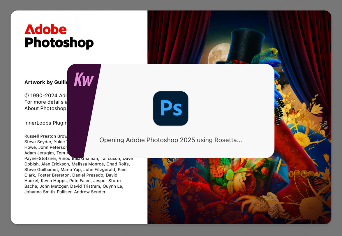
Kwiketta 2 launching Adobe Photoshop 2025
To be App Store compatible, we also had to find a way to replace the Dock Tile Plugin used for getting to the app’s settings when it’s not actually running. Kwiketta now uses special shortcuts on the Dock icon’s recent list for this purpose, available after the very first launch of the app.
Other than this, the functionality is identical to what I described in my original announcement post.
Kwiketta 2 fully supports the latest macOS and Photoshop versions.
Originally the app was coffee-supported, but we moved to the traditional upfront payment method with the App Store version. The price is still the same – around what you pay for a coffee – with a special introductory price until the end of November. Users who bought me a coffee for the original version should contact DIRE Studio for a replacement license.
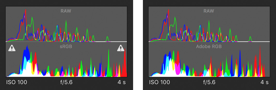
 So version 3.2 sports a new Dual Histogram tool to show Kuuvik Capture’s RAW histogram along the usual one generated from processed data.
 For the mathematically inclined, usable bit depth is calculated with the formula:


