Composing Stitched Images Made Easy

As you probably noticed from my posts, I’m a huge fan of Canon’s TS-E 24mm f/3.5L II lens. One of the reasons is that I can make pixel-perfectly stitch-able 2.4:1 wide panoramic shots – like the one below – with it. The only difficulty in making those images was composition: it isn’t easy to visualize a shot when you only see half of it.
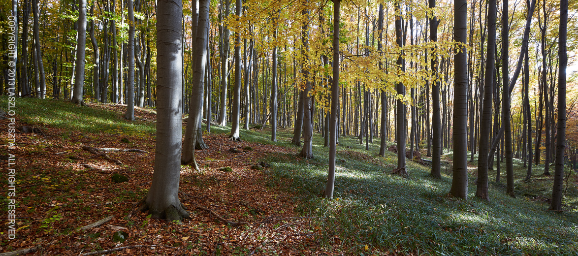
This image is a stitch of two frames: one taken with the lens shifted all the way to the left, while the other with the lens shifted to the right. Extreme edges cropped.

This image is a stitch of two frames: one taken with the lens shifted all the way to the left,
while the other with the lens shifted to the right. Extreme edges cropped.

But that difficulty is past now.

A couple of weeks ago I received a package from ALPA, containing their brand new ACAM Super Wide Converter. They sent it for certification with our upcoming Mark II Artist’s Viewfinder app, and also for my personal use. It was like Christmas for me. Quick first tests showed that the adapter has a conversion factor around 0.5x, which number was later confirmed with formal measurement in our lab. In other words, you can simulate a 17mm lens attached to a full frame 35mm using that. Or you can view almost the whole wide frame that will result from the TS-E stitch!

This is no small feat: you can walk around carrying a finder and checking lots of stitched composition without actually setting up the camera. And the actual capture needs less than half of the time it used to require.

The whole setup

The following image shows the setup I use for taking the images for pano stitches.
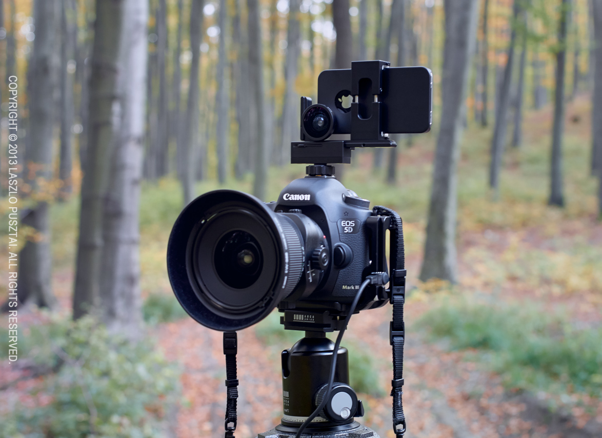
My stitched pano setup

My stitched pano setup

The camera and lens is nothing special, however the thing on top is. Attached to my iPhone is the ACAM wide adapter. The phone is held in position (note that the lenses are centered to avoid horizontal parallax) by an ALPA iPhone Holder. This is the Mark I, they now sell the Mark II complete with the wide angle adapter. As the holder was designed to be used on ALPA cameras, thus I also use an ALPA hot shoe mount adapter.

How much? – you might ask. You should log in to ALPA’s site to see their current prices, but as a guide: this whole viewfinder setup will set you back around $1150 (including the holder, hot shoe adapter, ACAM wide adapter and our Viewfinder iPhone app). If you think that’s a lot for a viewfinder, I recommend you to check out prices on a Linhof 45 Multifocus Viewfinder, for example (hint: it is around $2000 for way less functionality).

The ACAM wide adapter itself selling for less than $60 is extremely affordable considering what you get in exchange. I recommend every serious landscape and architecture photographer to check out this solution. Paired with our upcoming Mark II Artist’s Viewfinder it offers unprecedented value and functionality.

Update 11/20/2013

Today we announced the beta of Mark II Artist’s Viewfinder that sports real-time distortion correction for the ACAM SWC, making the above rig much more valuable. Read my post about it.
DoF Conversion Factor – The Exercise

In my previous post I described how easy it is to calculate apertures to get equivalent depth of field on different formats. I presented there all the equations needed for DoF calculation, but left the actual “paperwork” to you.

In this post I’ll do these calculations for those of you who did not do the homework ;)

Our goal is to get the same amount of depth of field for two setups. Object distance is also the same, so we can simply work with hyperfocal distances.

HfF2NFcFfC2NCcC

Where the index F denotes full frame and the C index denotes crop sensor cameras.

We also know how the required full frame and crop factor focal lengths relate (X denotes the crop factor), so:

X2fC2NFcFfC2NCcC

Now let’s see how the circle of confusion changes with the format. Having the exact same print dimensions, magnification will be higher for smaller formats.

mC=XmF

Viewing distance and your eye’s resolution are also the same, so:

cC=tan(π180Re)DvXmF

XcC=tan(π180Re)DvmF=cF

To summarize what we have:

X2fC2NFXcCfC2NCcC

Which after simplification leads to:

XNF1NC

That is, we arrive to the result:

XNCNF.

The Depth of Field Conversion Factor

It is widely known how sensor size influences angle of view (the value describing this called focal length conversion factor, or field of view conversion factor, or simply crop factor). But what about depth of field?

You won’t find too much literature on depth of field equivalence on different formats. This is possibly because the majority of DoF calculators are inherently flawed, and you can’t arrive at the correct result using them. More on this later – now let me ask you a question:

I photograph a scene with a full-frame 35mm camera using a 50mm lens. The lens is focused to 10m distance, and the aperture used is f/8. I will print the image at 30x45cm size. What lens and aperture should I use on an 1.6x crop factor APS-C sensor camera if I want the resulting print to look the same? By same I mean identical framing and identical depth of field. Of course both prints are viewed from the same distance.

Please spend a minute thinking about it before reading further.

:

Ok, now we can discuss the results!

The focal length part is easy: just divide the full-frame focal length by the crop factor.

50/1.6=31.25

I tell you the correct answer to the aperture part before delving into the the details. You should do the same: divide the full-frame aperture by the crop factor.

8/1.6=5

That is, you have to use a wider, 31.25mm lens and open up the aperture to f/5.

So the depth of field conversion factor is same as the crop factor. Frankly, this simplifies how one can quickly calculate it in the field.

The Math

I’ll let you do the actual calculations as an exercise (optionally you can read my solution here), but definitely want to talk about the correct way of calculating depth of field. We usually start with determining the hyperfocal distance H.

H=f2Nc+f

Where f is the lens’ focal length and N is the F-number. As the focal length is negligible compared to the hyperfocal distance, in practice we can safely use:

Hf2Nc

The problem child is c, which denotes the circle of confusion. No it’s not a group of photographers arguing about depth of field, this number represents the amount of blur on the sensor plane that is still perceived as sharp detail on the final print.

c=tan(π180Re)Dvm

Where Re is the resolution of the viewer’s eye expressed in cycles per degree, Dv is the viewing distance in millimeters, and m is the print’s magnification (calculated as the print’s linear dimension divided by the sensor’s linear dimension).

As you can see the circle of confusion depends on the print’s magnification, the viewing distance and the viewer’s eye condition. Any depth of field calculator that doesn’t let you input these values is just a waste of time. Actually those unusable calculators just take a fixed c for some smallish print size and less than 20/20 eye condition. But to arrive at the correct depth of field equivalence factor you have to begin with a correct c.

Note that sensor resolution does not play a role in circle of confusion and thus depth of field. It limits maximum magnification (that still looks good), however.

From here the near and far depth of field is calculated with the following equations (or their approximations).

DoFn=HsH+(sf)HsH+s

DoFf=HsH(sf)HsHs for s<H

Where s is the subject distance.

Interesting Consequences

Diffraction limited depth of field is the same for any two sensors having the same number of megapixels. Even if they have different diffraction limited apertures. That is, the diffraction limited aperture is an 1.6x smaller F-number for an 1.6x crop factor camera than for an equal megapixel full frame camera.

f/5.6 maximum aperture zoom lenses on APS-C cameras are a joke. Who would want to shoot with a f/9 lens on a full frame camera?!?

You need wider maximum aperture lenses on APS-C cameras than you would on full frame. The new Sigma 18-35 f/1.8 lens is a good step in this direction.

You can capture the exact same looking image on an APS-C crop sensor camera that you could on a full frame one. You’ll just need a wider, faster (and higher resolution and more expensive) lens.

How to Make Focusing a Tilt/Shift Lens Easier

The tilt movement is used in technical cameras as well as DSLR tilt/shift lenses to precisely adjust where the plane of focus is on the image. Focusing with tilt is a tedious process (described here and here), but the results always worth the time!

There was a big pain point in using DSLR T/S lenses: checking what you have done. The viewfinder isn’t enough for that with today’s high resolution bodies, so you have to zoom in and check different points on the image using magnified live view. The adjust either tilt or focus. Then check the points. Then refocus… I had some images where I spent more than half an hour on fine tuning focus!

I said “was” – as it was the case before Kuuvik Capture’s Split View feature came along. I’m using this since I was halfway into developing the first prototype, and man, it can save lots of time! No, it won’t think instead of you, but the ability to quickly and visually asses what you have accomplished is priceless. It is also a great tool for learning how to focus a tilt/shift lens.

So watch the video below, and if you are using a Canon EOS-1D X, 5D Mark III or 6D with any of Canon’s great tilt/shift lenses, then grab Kuuvik Capture’s beta now! It’s that good (OK, don’t believe me, try it for yourself ;)).

Click here to watch it on our YouTube channel.

The Adventure of the Mendacious Histogram

Digital exposure optimization is a controversial topic. Although the notion of “exposing to the right” is widespread, widely accepted with a large group of advocates, camera manufacturers “doesn’t seem to get it”. But there’s much more technical stuff behind this than simple ignorance. In this post I’ll shed some light on how complicated digital exposure optimization could be.

Let’s start with ETTR. Two of my masters, Michael Reichmann and Jeff Schewe had extensively written about the topic, so instead of replicating it I would encourage you to read the following articles and Jeff’s new book. It is imperative to grasp the idea so that you can understand the rest of the post.

  • Expose (to the) Right – The original article from 2003.
  • Optimizing Exposure – A rather utopistic view of the problem. Reminds me of Adams’ (Douglas, not Ansel) Total Perspective Vortex – as it extrapolates a whole universe not from a fairy cake, but from the fact that increasing exposure reduces shadow noise. Anyway, a good read on what would be really needed from a photographers point of view, even if its not possible with the current technology.
  • The Digital Negative – Jeff’s book collects the majority of information about digital exposure right in its first chapter.

To summarize: increasing exposure has advantages to the shadows and the amount of information retained in the RAW file. That’s great. But here comes the million dollar question: how much one should increase exposure being hundred percent confident that highlights aren’t blown or destroyed (and thus, keeping all the possible information)? You should read Ctein’s article on the dangers of ETTR regarding lost highlights.

I hope you are confused enough about whether to ETTR or not and how can you really assess over-exposure. Don’t be afraid, this is the where our adventure begins.

Before we embark on it, let me rephrase the question: as overexposure is terminal to the data (details) in the overexposed area, how can one avoid it with confidence? Regardless of whether you ETTR or not, this is important. Imagine a bright yellow flower for example. Overexposing one or more channels will destroy fine color variance – which is a bad thing (except if you will run the image through some ugly lo-fi filter, of course, in which case the things I’m writing about is totally unimportant to you). Also, what I’m writing about is for RAW shooters only. JPEG guys only get what they see, so these topics does not apply to them.

Let’s begin!

One Image – Three (Different) Histograms

The histogram is the primary tool for assessing exposure on a digital camera. But what your camera shows has only a little resemblance to the RAW data recorded. This is because all JPEG settings, such as white balance, color space, sharpening, contrast, etc. influence the histogram display. As a result, the histogram on the LCD comes from the JPEG preview of your RAW file. In an ideal world, one could set the histogram into “RAW mode” which would instruct the camera to calculate the histogram from the RAW data instead of the JPEG preview.

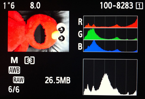
Canon 5D III, Auto WB

The majority of the parameters mentioned above can be zeroed (like sharpening, contrast) on the camera. The problem-child is white balance, where we have little influence by default.

Take the image on the left, for example. The RGB histogram shows gross overexposure in the red channel, you can even see overexposure warning “blinkies” in Elmo’s eyes.

Based on the camera’s histogram one would lower the exposure to avoid overexposing Elmo’s… wait! Blinkies warn for overexposure in the eyes, not the red fur, even if the red channel was blown. Something isn’t kosher with this…

Histogram from RAW Data

On the right is a histogram generated from the same image with Kuuvik Capture utilizing gamma-corrected RAW data. As you can see reds are far from being overexposed. You can also see a different distribution in the RAW histogram, with the peaks are being at distinctly different places. This is because the RAW histogram in KCapture is not white balanced.

White balance is set by multiplying data coming from a channel with a number (the white balance coefficient) to “scale” it to reach the desired white point. It is represented by a four element vector (one number for each channel, in RGGB order). You can use exiftool to examine these coefficients, they are displayed as WB RGGB Levels As Shot. The actual values for the above image are: (2185, 1024, 1024, 1526). That is, you have to multiply the red channel by 2185/1024 = 2.13 to get the white balanced image. You can easily see from the RAW histogram that multiplying reds by 2.13 on this image will blow the channel out – in that white balance setting.

Sidebar: white balance is always represented as RGGB coefficients internally, not with color temperature/tint as RAW converters and cameras present this data to you. Color temperature is an “artificial” construct to handle these numbers in a more user-friendly way. And the way these coefficients are converted into color temperature is a proprietary process for each converter. This is why you get completely different white by using the same Kelvin value in different converters.

Now let’s take a look on what RAW converters, Adobe Camera RAW 7.3 to be exact, think about the same image (Capture One displays a similar one).

Histogram in ACR 7

Part of the black magic of RAW conversion is graceful handling of the roll-off into overexposure. The fact that a non-overexposed channel can be blown during white balancing is responsible for the converter’s ability to do highlight recovery. They are mostly taming the data that is blown only by the currently set white balance. As the common myth goes: RAW files have more headroom in the highlights. And as with most of the myths, there is truth lurking behind it: because the white balance is not fixed in RAW captures, converters have the ability to extract more information from it than you would be able to get from a JPEG, where clipped highlights (even if clipped by the current white balance setting) are lost forever.

Above I shown you the case when the JPEG histogram shows overexposure, while the RAW histogram doesn’t. It could happen the other way around, which is even more dangerous. I recommend you to read Alex Tutbalin’s article on white balancing problems for an example. Alex is the author of Libraw, the library Kuuvik Capture is also using for extracting RAW data from proprietary file formats, such as Canon’s CR2.

On Gamma Correction

If you read Alex’s article, you saw the Rawnalyze tool, and if you try both that and Kuuvik Capture, you’ll get different histograms. Why? Because what Rawnalyze displays is the rawest raw data possible. That is, it doesn’t map the camera’s black level to the left side and the maximum saturation level on a given ISO to the right of the histogram (in other words, it does not scale the data). In KCapture I wanted to make the RAW histogram to look familiar to photographers (including myself), so instead of blindly displaying the raw data the app does a little processing. The processing consists of scaling (so black is on the left and white is on the right instead of somewhere in the middle of the histogram), and gamma correction.

By default RAW data is linear, that is the highest exposure stop occupies the entire right half of the histogram, the next 1/4 of it, and so on. The result is that a linear RAW histogram pushes all the data to the left, and makes it hard to judge shadow exposure and see whether we have a clipping there. Instead KCapture corrects this data the same way it happens during RAW conversion: by applying a gamma curve to make exposure stops equal sized on the display.

Mapping Theory to Practice

Let’s draw some conclusions. First, 1) white balanced in-camera histograms are not suitable for checking overexposure. RAW histograms are markedly better in this, but 2) RAW histograms can only show physical overexposure of channel(s), and are blind to white balancing induced highlight clipping. Most of that clipping is curable in the converter utilizing some form of highlight recovery, however. The 3) final word on highlight clipping is said by the RAW converter after white balance has been set.

(2) is why I called Michael’s second article an utopia. When we wrote the specification for Kuuvik Capture back in December 2011, our goal was to implement ETTR optimization described in that article. It turned out rather quickly that you can’t do this unless you have the final white balance set – which will not happen until later in the process. And even if you can do this, you shouldn’t always ETTR. Sometimes artificially overexposed images will push the noise from the shadows into the sky (scroll down to the ETTR section in the linked article for an example). And even ETTR could be behind skies turning purple.

(3) is the real reason why camera manufacturers are unable to show the same histogram as your converter (unless they are using the same algorithms, of course – which is highly unlikely).

So how do I use this information in practice?

When I’m shooting tethered (which is the majority of cases when I do landscape work), I rely on Kuuvik Capture to check the physical exposure from RAW histograms. If your physical exposure is bad it won’t get any better during RAW conversion. What I look for here is potentially uncorrectable overexposure (non-specular highlights) and as a Canon shooter who’s cursed with muddy shadows, I check for underexposure. I usually push the exposure to the right when the shadows are in danger or when there’s plenty of room for the highlights.

Then I pass the image to Capture One for the final decision. Capture One 6 had some issues with highlight roll-off handling with the 5D3, so I had to back-off a bit from extreme highlights, but v7 fixes this problem (be sure to use the v7 process).

Free (that is, non-tethered) shooting is a different beast. One needs a trick to cancel the side effects of white balancing.

Unitary White Balance

Guillermo Luijk came up with the idea of UniWB in 2008. UniWB is basically a custom white balance that sets the WB coefficients to 1 (hence the name unitary). It could be useful in the field if you can live with the ugly green images (to avoid that I usually just use UniWB for exposure tuning and switch back to AWB for the real shot).

The real downside of UniWB was the tedious process of obtaining the magenta target image. Having control over the WB coefficients, you can obtain the UniWB setting in Kuuvik Capture just with two clicks: on the Set Unitary White Balance item on the Camera menu.

Making “The First Flower” with Kuuvik Capture

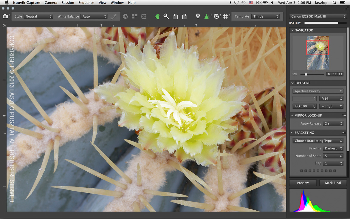
As I told you in the introduction of Kuuvik Capture, I used the software yesterday for shooting quasi-macros with the Canon 135 f/2. In this post I’ll give a detailed description how it helped me creating The First Flower.

Checking sharpness and histogram. Click the image for a larger version.

The final optimized image. Click the image for a larger version.

The biggest challenge was keeping the appropriate depth of field, without the softening effect of diffraction. I would like to expose the image at f/11 or wider, so I focused on the flower and checked the image in 5x magnification to see whether all the thorns are in focus. Unfortunately they weren’t. So I placed a marker on the flower, and another one on the lower left part of the image and entered split view. Split view can show you two or three 5x magnified parts of the image simultaneously with the 5D Mark III.

Why just 5x and not 10x? Simply because 10x is an “empty magnification” in Canons, that is you do not get more detail in 10x. This is because the 10x magnification is simply the 5x image blown up in software!

Seeing both parts at once I was able to see how much more should I stop down. I used depth of field preview and focus pulling to optimize sharpness for the thorns. I ended up shooting the first preview at f/14. Critical focus check at 100% revealed just a tiny bit of softness at the base of the thorns on the lower left, so I stopped down to f/16 and took another preview. It was good at this time.

Then came exposure optimization. I started out at +1 during the live view part, and seeing the raw histogram I knew that I have some more headroom to lighten the image, thus keep more data. At +1 2/3 stops the image became overexposed, so I lowered the exposure to +1 1/3.

Deleted the markers and turned off focus peaking to see the image in its entirety, it was what I was after (this is what you can see on the above screenshot). I marked it final. This step removed all four preview images I made during the optimization – both from the computer and from the camera’s memory card. In the studio I didn’t have to go through the selection process as I just had a single, final, optimized image.